Introduction to R
Summer Training for Research Scholar Program
Installation
- Install R using appropriate link from The Comprehensive R Archive Network.
- Download and install RStudio for free. Just click the “Download RStudio” button and follow instructions.
Basics
When you type a command at the prompt of the Console window and hit Enter, your computer executes the command and shows you the results. Then RStudio displays a new prompt for your next command. For example, if you type 2 + 3 and hit Enter, RStudio will display:
2 + 3[1] 5or
21 / (4 + 3) [1] 3You can use common functions, like log(), sin(), cos() and many others:
log(2)[1] 0.6931472Objects (or variables)
You can assign values to R objects using <- symbol:
height <- 70R is case sensitive, so variables Height and height are two distinct objects.
You can define an R object, that stores multiple values. For example, you can create a vector that contains a sequence of integer values (notice that both - start and end values are included):
id <- 1:10
id
[1] 1 2 3 4 5 6 7 8 9 10Avoid using names c, t, cat, F, T, D as those are built-in functions/constants.
The variable name can contain letters, digits, underscores and dots and start with the letter or dot. The variable name cannot contain dollar sign or other special characters.
str.var  <- "oxygen"               # character variable
num.var  <- 15.99                  # numerical variable
bool.var <- TRUE                   # Boolean (or logical) variable
bool.var.1 <- F                    # logical values can be abbreviated
Vectors
Vector is an array of values of the same type: Vectors can be numeric, character or logical:
# Function c() is used to create a vector from a list of values
num.vector <- c( 5, 7, 9, 11, 4, -1, 0)

# Numeric vectors can be defined in a number of ways:
vals1 <- c (2, -7, 5, 3, -1 )             # concatenation
vals2 <- 25:75                            # range of values
vals3 <- seq(from=0, to=3, by=0.5)        # sequence definition
vals4 <- rep(1, times=7)                  # repeat value
vals5 <- rnorm(5, mean=2, sd=1.5 )        # normally distributed values
R Functions
There are many functions that come with R installation:
mean(1:99)[1] 50R Help
You can access the function’s help topic in two ways:
?sd
help(sd)
If you do not know the function’s name, you can search for a topic
??"standard deviation"
help.search("standard deviation")
Installing R packages
There are more than 20 thousand packages published officially on the CRAN’s website. You can search them by name or by topic.
There are also many packages published on the Bioconductor site
To install an R package from the CRAN, use install.packages("package_name") command. For example, you may want to install a very popular tidyverse library of packages used by many data scientists:
install.packages("tidyverse")Another very handy package is table1:
# To install package
install.packages("table1")
Once package is installed it can be loaded and used:
#Load R package
library(table1)
Vector operations in R
# Define a vector with values of body temperature in Fahrenheit
ftemp <- c(97.8, 99.5, 97.9, 102.1, 98.4, 97.7)

# Convert them to a vector with values in Celsius
ctemp <- (ftemp - 32) / 9 * 5
print(ctemp)
[1] 36.55556 37.50000 36.61111 38.94444 36.88889 36.50000You can also perform operations on two or more vectors:
# Define values for body weight and height (in kg and meters)
weight <- c(65, 80, 73, 57, 84)
height <- c( 1.65, 1.80, 1.73, 1.68, 1.79)

# Calculate BMI
weight/height^2
[1] 23.87511 24.69136 24.39106 20.19558 26.21641Vector Slicing (subsetting)
x <- c(36.6, 38.2, 36.4, 37.9, 41.0, 39.9, 36.8, 37.5)
x[2]         # returns second element
[1] 38.2x[2:4] # returns 2nd through 4th elements inclusive[1] 38.2 36.4 37.9x[c(1,3,5)] # returns 1st, 3rd and 5th elements[1] 36.6 36.4 41.0# compare each element of the vector with a value
x < 37.0[1] TRUE FALSE TRUE FALSE FALSE FALSE TRUE FALSE# return only those elements of the vector that satisfy a specific condition
x[ x < 37.0 ] [1] 36.6 36.4 36.8There are a number of functions that are useful to locate a value satisfying specific condition(s)
which.max(x) # find the (first)maximum element and return its index[1] 5which.min(x)[1] 3which(x >= 37.0) # find the location of all the elements that satisfy a specific condition[1] 2 4 5 6 8Useful Functions:
max(x),   min(x),   sum(x)
mean(x),  sd(), median(x),  range(x)
var(x)                            - simple variance
cor(x,y)                          - correlation between x and y
sort(x), rank(x), order(x)        - sorting
duplicated(x), unique(x)          - unique and repeating values
summary()
Missing Values
Missing values in R are indicated with a symbol NA:
x <- c(734, 145, NA, 456, NA)

# check if there are any missing values:
anyNA(x)
[1] TRUETo check which values are missing use is.na() function:
is.na(x) # check if the element in the vector is missing[1] FALSE FALSE TRUE FALSE TRUEwhich(is.na(x)) # which elements are missing[1] 3 5By default statistical functions will not compute if the data contain missing values:
mean(x)[1] NATo view the arguments that need to be used to remove missing data, read help topic for the function:
?mean#Perform computation removing missing data
mean(x, na.rm=TRUE)[1] 445Reading input files
There are many R functions to process files with various formats: Some come from base R:
- read.table()
- read.csv()
- read.delim()
- read.fwf()
- scan() and many others
# Read a regular csv file:
salt <- read.csv("http://rcs.bu.edu/classes/STaRS/intersalt.csv")
There are a few R packages which provide additional functionality to read files.
# Install package first
# You can install packages from the RStudio Menu (Tools -> Install packages)
#    or by executing the following R command:
#install.packages("foreign")

#Load R package "foreign"
library(foreign)

# Read data in Stata format
swissdata <- read.dta("http://rcs.bu.edu/classes/STaRS/swissfile.dta")

# Load R package haven to read SAS-formatted files (make sure it is installed! )
#install.packages("haven")
library(haven)

# Read data in SAS format
fhsdata <- read_sas("http://rcs.bu.edu/classes/STaRS/fhs.sas7bdat")
Exploring R dataframes
There are a few very useful commands to explore R’s dataframes:
head(fhsdata)# A tibble: 6 × 13
SEX RANDID TOTCHOL AGE SYSBP DIABP DIABETES BPMEDS PERIOD CIGPDAY HEARTRTE
<dbl> <dbl> <dbl> <dbl> <dbl> <dbl> <dbl> <dbl> <dbl> <dbl> <dbl>
1 1 2448 195 39 106 70 0 0 1 0 80
2 1 2448 209 52 121 66 0 0 3 0 69
3 2 6238 250 46 121 81 0 0 1 0 95
4 2 6238 260 52 105 69.5 0 0 2 0 80
5 2 6238 237 58 108 66 0 0 3 0 80
6 1 9428 245 48 128. 80 0 0 1 20 75
# ℹ 2 more variables: HDLC <dbl>, LDLC <dbl>tail(fhsdata)# A tibble: 6 × 13
SEX RANDID TOTCHOL AGE SYSBP DIABP DIABETES BPMEDS PERIOD CIGPDAY HEARTRTE
<dbl> <dbl> <dbl> <dbl> <dbl> <dbl> <dbl> <dbl> <dbl> <dbl> <dbl>
1 1 1.00e7 185 40 141 98 0 0 1 0 67
2 1 1.00e7 173 46 126 82 0 0 2 0 70
3 1 1.00e7 153 52 143 89 0 0 3 0 65
4 2 1.00e7 196 39 133 86 0 0 1 30 85
5 2 1.00e7 240 46 138 79 0 0 2 20 90
6 2 1.00e7 NA 50 147 96 0 0 3 10 94
# ℹ 2 more variables: HDLC <dbl>, LDLC <dbl>str(fhsdata)tibble [11,627 × 13] (S3: tbl_df/tbl/data.frame)
$ SEX : num [1:11627] 1 1 2 2 2 1 1 2 2 2 ...
$ RANDID : num [1:11627] 2448 2448 6238 6238 6238 ...
..- attr(*, "label")= chr "Random ID"
$ TOTCHOL : num [1:11627] 195 209 250 260 237 245 283 225 232 285 ...
$ AGE : num [1:11627] 39 52 46 52 58 48 54 61 67 46 ...
$ SYSBP : num [1:11627] 106 121 121 105 108 ...
$ DIABP : num [1:11627] 70 66 81 69.5 66 80 89 95 109 84 ...
$ DIABETES: num [1:11627] 0 0 0 0 0 0 0 0 0 0 ...
$ BPMEDS : num [1:11627] 0 0 0 0 0 0 0 0 0 0 ...
$ PERIOD : num [1:11627] 1 3 1 2 3 1 2 1 2 1 ...
..- attr(*, "label")= chr "Examination cycle"
$ CIGPDAY : num [1:11627] 0 0 0 0 0 20 30 30 20 23 ...
..- attr(*, "label")= chr "Cigarettes per day"
$ HEARTRTE: num [1:11627] 80 69 95 80 80 75 75 65 60 85 ...
..- attr(*, "label")= chr "Ventricular Rate (beats/min)"
$ HDLC : num [1:11627] NA 31 NA NA 54 NA NA NA NA NA ...
..- attr(*, "label")= chr "HDL Cholesterol mg/dL"
$ LDLC : num [1:11627] NA 178 NA NA 141 NA NA NA NA NA ...
..- attr(*, "label")= chr "LDL Cholesterol mg/dL"summary(fhsdata) SEX RANDID TOTCHOL AGE
Min. :1.000 Min. : 2448 Min. :107.0 Min. :32.00
1st Qu.:1.000 1st Qu.:2474378 1st Qu.:210.0 1st Qu.:48.00
Median :2.000 Median :5006008 Median :238.0 Median :54.00
Mean :1.568 Mean :5004741 Mean :241.2 Mean :54.79
3rd Qu.:2.000 3rd Qu.:7472730 3rd Qu.:268.0 3rd Qu.:62.00
Max. :2.000 Max. :9999312 Max. :696.0 Max. :81.00
NA's :409
SYSBP DIABP DIABETES BPMEDS
Min. : 83.5 Min. : 30.00 Min. :0.00000 Min. :0.0000
1st Qu.:120.0 1st Qu.: 75.00 1st Qu.:0.00000 1st Qu.:0.0000
Median :132.0 Median : 82.00 Median :0.00000 Median :0.0000
Mean :136.3 Mean : 83.04 Mean :0.04558 Mean :0.5402
3rd Qu.:149.0 3rd Qu.: 90.00 3rd Qu.:0.00000 3rd Qu.:0.0000
Max. :295.0 Max. :150.00 Max. :1.00000 Max. :9.0000
PERIOD CIGPDAY HEARTRTE HDLC
Min. :1.000 Min. : 0.00 Min. : 37.00 Min. : 10.00
1st Qu.:1.000 1st Qu.: 0.00 1st Qu.: 69.00 1st Qu.: 39.00
Median :2.000 Median : 0.00 Median : 75.00 Median : 48.00
Mean :1.899 Mean : 14.98 Mean : 77.26 Mean : 49.37
3rd Qu.:3.000 3rd Qu.: 20.00 3rd Qu.: 85.00 3rd Qu.: 58.00
Max. :3.000 Max. :999.00 Max. :999.00 Max. :189.00
NA's :8600
LDLC
Min. : 20.0
1st Qu.:145.0
Median :173.0
Mean :176.5
3rd Qu.:205.0
Max. :565.0
NA's :8601 # In this dataset, "999" is used to indicate missing values
fhsdata$HEARTRTE[fhsdata$HEARTRTE==999]<- NA
fhsdata$CIGPDAY[fhsdata$CIGPDAY==999]<- NA
summary(fhsdata) SEX RANDID TOTCHOL AGE
Min. :1.000 Min. : 2448 Min. :107.0 Min. :32.00
1st Qu.:1.000 1st Qu.:2474378 1st Qu.:210.0 1st Qu.:48.00
Median :2.000 Median :5006008 Median :238.0 Median :54.00
Mean :1.568 Mean :5004741 Mean :241.2 Mean :54.79
3rd Qu.:2.000 3rd Qu.:7472730 3rd Qu.:268.0 3rd Qu.:62.00
Max. :2.000 Max. :9999312 Max. :696.0 Max. :81.00
NA's :409
SYSBP DIABP DIABETES BPMEDS
Min. : 83.5 Min. : 30.00 Min. :0.00000 Min. :0.0000
1st Qu.:120.0 1st Qu.: 75.00 1st Qu.:0.00000 1st Qu.:0.0000
Median :132.0 Median : 82.00 Median :0.00000 Median :0.0000
Mean :136.3 Mean : 83.04 Mean :0.04558 Mean :0.5402
3rd Qu.:149.0 3rd Qu.: 90.00 3rd Qu.:0.00000 3rd Qu.:0.0000
Max. :295.0 Max. :150.00 Max. :1.00000 Max. :9.0000
PERIOD CIGPDAY HEARTRTE HDLC
Min. :1.000 Min. : 0.00 Min. : 37.00 Min. : 10.00
1st Qu.:1.000 1st Qu.: 0.00 1st Qu.: 69.00 1st Qu.: 39.00
Median :2.000 Median : 0.00 Median : 75.00 Median : 48.00
Mean :1.899 Mean : 8.25 Mean : 76.78 Mean : 49.37
3rd Qu.:3.000 3rd Qu.:20.00 3rd Qu.: 85.00 3rd Qu.: 58.00
Max. :3.000 Max. :90.00 Max. :220.00 Max. :189.00
NA's :79 NA's :6 NA's :8600
LDLC
Min. : 20.0
1st Qu.:145.0
Median :173.0
Mean :176.5
3rd Qu.:205.0
Max. :565.0
NA's :8601 We can use table1 package to get various summaries stratifying by one or more variable:
# One level of stratification
table1(~ SEX + AGE + TOTCHOL | DIABETES, data=fhsdata)| 0 (N=11097) |
1 (N=530) |
Overall (N=11627) |
|
|---|---|---|---|
| SEX | |||
| Mean (SD) | 1.57 (0.495) | 1.52 (0.500) | 1.57 (0.495) |
| Median [Min, Max] | 2.00 [1.00, 2.00] | 2.00 [1.00, 2.00] | 2.00 [1.00, 2.00] |
| AGE | |||
| Mean (SD) | 54.5 (9.52) | 60.8 (8.54) | 54.8 (9.56) |
| Median [Min, Max] | 54.0 [32.0, 81.0] | 61.0 [36.0, 80.0] | 54.0 [32.0, 81.0] |
| TOTCHOL | |||
| Mean (SD) | 241 (44.9) | 242 (53.6) | 241 (45.4) |
| Median [Min, Max] | 238 [107, 696] | 236 [112, 638] | 238 [107, 696] |
| Missing | 381 (3.4%) | 28 (5.3%) | 409 (3.5%) |
# Two levels of stratification (nesting)
table1(~ AGE + TOTCHOL + HDLC | DIABETES*SEX, data=fhsdata)
0
|
1
|
Overall
|
||||
|---|---|---|---|---|---|---|
| 1 (N=4769) |
2 (N=6328) |
1 (N=253) |
2 (N=277) |
1 (N=5022) |
2 (N=6605) |
|
| AGE | ||||||
| Mean (SD) | 54.2 (9.49) | 54.7 (9.53) | 59.8 (8.39) | 61.7 (8.59) | 54.5 (9.51) | 55.0 (9.60) |
| Median [Min, Max] | 54.0 [33.0, 80.0] | 54.0 [32.0, 81.0] | 60.0 [39.0, 79.0] | 62.0 [36.0, 80.0] | 54.0 [33.0, 80.0] | 55.0 [32.0, 81.0] |
| TOTCHOL | ||||||
| Mean (SD) | 235 (42.4) | 246 (46.2) | 228 (42.8) | 255 (59.4) | 234 (42.4) | 247 (46.9) |
| Median [Min, Max] | 232 [113, 696] | 243 [107, 625] | 230 [115, 366] | 248 [112, 638] | 232 [113, 696] | 243 [107, 638] |
| Missing | 100 (2.1%) | 281 (4.4%) | 7 (2.8%) | 21 (7.6%) | 107 (2.1%) | 302 (4.6%) |
| HDL Cholesterol mg/dL | ||||||
| Mean (SD) | 43.7 (13.1) | 54.0 (15.8) | 43.8 (15.2) | 49.3 (17.1) | 43.7 (13.3) | 53.6 (15.9) |
| Median [Min, Max] | 42.0 [10.0, 138] | 52.0 [11.0, 189] | 41.0 [17.0, 118] | 48.0 [15.0, 93.0] | 42.0 [10.0, 138] | 52.0 [11.0, 189] |
| Missing | 3578 (75.0%) | 4724 (74.7%) | 140 (55.3%) | 158 (57.0%) | 3718 (74.0%) | 4882 (73.9%) |
To see more examples of table1 package usage, see. https://cran.r-project.org/web/packages/table1/vignettes/table1-examples.html
Correlation
To explain this test, we will use the salt dataset we imported earlier:
str(salt)'data.frame': 52 obs. of 4 variables:
$ b : num 0.512 0.226 0.316 0.042 0.086 0.265 0.384 0.501 0.352 0.443 ...
$ bp : num 72 78.2 73.9 61.7 61.4 73.4 79.2 66.6 82.1 75 ...
$ sodium : num 149.3 133 142.6 5.8 0.2 ...
$ country: chr "Argentina" "Belgium" "Belgium" "Brazil" ...The correlation test is used to test the linear relationship of 2 continuous variables. We can first display two variables using scatter plot:
plot(x = salt$sodium,
     y = salt$bp,
     xlab = "mean sodium excretion (mmol/24h)",
     ylab = "mean diastolic blood pressure (mm Hg)",
     main = "Diastolic Blood Presure vs Sodium excretion")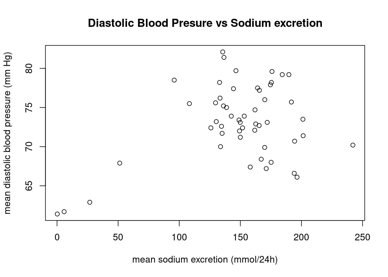
As we can see in this plot, there is little correlation between these 2 variables and there are a few “outlier” points that will affect the correlation calculation!!!
Let’s perform the test:
cor.test(salt$bp, salt$sodium)
    Pearson's product-moment correlation

data:  salt$bp and salt$sodium
t = 2.7223, df = 50, p-value = 0.008901
alternative hypothesis: true correlation is not equal to 0
95 percent confidence interval:
 0.09577287 0.57573339
sample estimates:
      cor
0.3592828
The Null Hypothesis : the true correlation between bp and sodium (blood pressure and salt intake) is 0 (they are independent);
The Alternative hypothesis: true correlation between bp and sodium is not equal to 0.
The p-value is less that 0.05 and the 95% CI does not contain 0, so at the significance level of 0.05 we reject null hypothesis and state that there is some (positive) correlation (0.359) between these 2 variables.
*  0 < |r| <= .3 - weak correlation
* .3 < |r| <= .7 - moderate correlation
*      |r| >  .7 - strong correlation
Important:
- The order of the variables in the test is not important
- Correlation provide evidence of association, not causation!
- Correlation values is always between -1 and 1 and does not change if the units of either or both variables change
- Correlation describes linear relationship
- Correlation is strongly affected by outliers (extreme observations)
In this case the correlation is weak and there are a few points that significantly affect the result.
Linear Model
lm.res <- lm( bp ~ sodium, data = salt)
summary(lm.res)
Call:
lm(formula = bp ~ sodium, data = salt)

Residuals:
    Min      1Q  Median      3Q     Max
-8.8625 -2.8906  0.0299  3.6470  9.4283

Coefficients:
            Estimate Std. Error t value Pr(>|t|)
(Intercept) 67.56245    2.14643  31.477   <2e-16 ***
sodium       0.03768    0.01384   2.722   0.0089 **
---
Signif. codes:  0 '***' 0.001 '**' 0.01 '*' 0.05 '.' 0.1 ' ' 1

Residual standard error: 4.511 on 50 degrees of freedom
Multiple R-squared:  0.1291,    Adjusted R-squared:  0.1117
F-statistic: 7.411 on 1 and 50 DF,  p-value: 0.008901
Here we estimated that relationship between the predictor (sodium) and response (bp) variables.
The summary statistics here reports a number of things. p-value tells us if the model is statistically significant.
In Linear Regression, the Null Hypothesis is that the coefficient associated with the variables are equal to zero.
Multiple R-squared value is equal to the square of the correlation value we calculated in the previous test.
When the model fits the data;
- R-squared - The higher - the better
- F-statistics - The higher the better
- Std. Error - The closer to 0 - the better
One Sample t-Test
This test is used to test the mean of a sample from a normal distribution
t.test(salt$bp, mu=70)
    One Sample t-test

data:  salt$bp
t = 4.7485, df = 51, p-value = 1.703e-05
alternative hypothesis: true mean is not equal to 70
95 percent confidence interval:
 71.81934 74.48451
sample estimates:
mean of x
 73.15192
The null hypothesis: The true mean is equal to 70. The alternative hypothesis: true mean is not equal to 70. Since p-value is small (1.703e-05) - less than 0.05, 95% percent CI does not contain the value 70, we can reject the null hypothesis.
Two Sample t-TEST
Let’s load some other dataset. It comes with R. This dataset shows the effect of two soporific drugs (increase in hours of sleep compared to control) on 10 patients. There are 3 variables:
- extra: (numeric) increase in hours of sleep.
- group: (factor) categorical variable indicating which drug is given
- ID: (factor) patient ID
data(sleep)
head(sleep)
extra group ID
1 0.7 1 1
2 -1.6 1 2
3 -0.2 1 3
4 -1.2 1 4
5 -0.1 1 5
6 3.4 1 6summary(sleep) extra group ID
Min. :-1.600 1:10 1 :2
1st Qu.:-0.025 2:10 2 :2
Median : 0.950 3 :2
Mean : 1.540 4 :2
3rd Qu.: 3.400 5 :2
Max. : 5.500 6 :2
(Other):8 To compare the means of 2 samples:
boxplot(extra ~ group, data = sleep)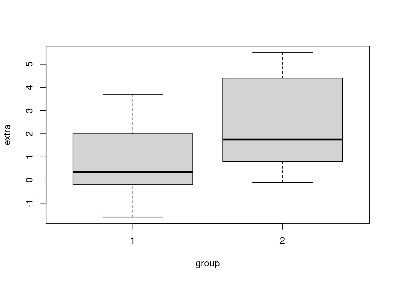
t.test(extra ~ group, data = sleep)
    Welch Two Sample t-test

data:  extra by group
t = -1.8608, df = 17.776, p-value = 0.07939
alternative hypothesis: true difference in means between group 1 and group 2 is not equal to 0
95 percent confidence interval:
 -3.3654832  0.2054832
sample estimates:
mean in group 1 mean in group 2
           0.75            2.33
Here the Null Hypothesis is that the true difference between 2 groups is equal to 0
And the Alternative Hypothesis is that it does not equal to 0 In this test the p-value is above significance level of 0.05 and 95% CI contains 0, so we cannot reject the NULL hypothesis.
Note, that t.test has a number of options, including alternative which can be set to “two.sided”, “less”, “greater”, depending which test you would like to perform. Using option var.equal you can also specify if the variances of the values in each group are equal or not.
One-way ANOVA test
The one-way analysis of variance (ANOVA) test is an extension of two-samples t.test for comparing means for datasets with more than 2 groups.
Assumptions:
- The observations are obtained independently and randomly from the population defined by the categorical variable
- The data of each category is normally distributed
- The populations have a common variance.
data("PlantGrowth")
head(PlantGrowth)
weight group
1 4.17 ctrl
2 5.58 ctrl
3 5.18 ctrl
4 6.11 ctrl
5 4.50 ctrl
6 4.61 ctrlsummary(PlantGrowth) weight group
Min. :3.590 ctrl:10
1st Qu.:4.550 trt1:10
Median :5.155 trt2:10
Mean :5.073
3rd Qu.:5.530
Max. :6.310 boxplot(weight~group, data=PlantGrowth)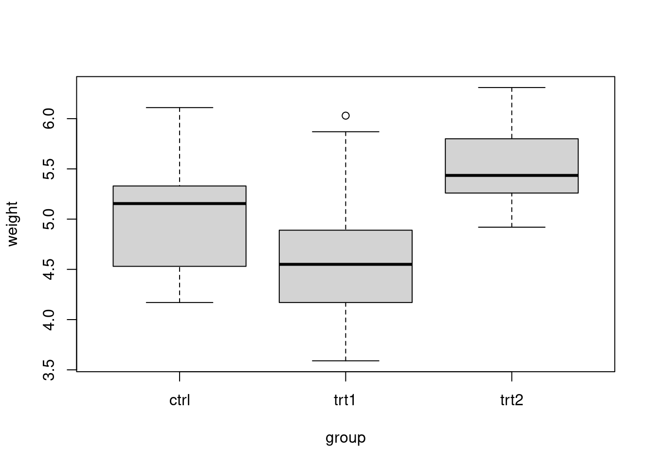
As visible from the side-by-side boxplots, there is some difference in the weights of 3 groups, but we cannot determine from the plot if this difference is significant.
aov.res <- aov(weight~group, data=PlantGrowth)
summary( aov.res )
Df Sum Sq Mean Sq F value Pr(>F)
group 2 3.766 1.8832 4.846 0.0159 *
Residuals 27 10.492 0.3886
---
Signif. codes: 0 '***' 0.001 '**' 0.01 '*' 0.05 '.' 0.1 ' ' 1As we can see from the summary output the p-value is 0.0159 < 0.05 which indicates that there is a statistically significant difference in weignt between these groups. We can check the confidence intervals for the treatment parameters:
confint(aov.res) 2.5 % 97.5 %
(Intercept) 4.62752600 5.4364740
grouptrt1 -0.94301261 0.2010126
grouptrt2 -0.07801261 1.0660126Important: In one-way ANOVA test a small p-value indicates that some of the group means are different, but it does not say which ones!
For multiple pairwise-comparisions we use Tukey test:
TukeyHSD(aov.res) Tukey multiple comparisons of means
95% family-wise confidence level
Fit: aov(formula = weight ~ group, data = PlantGrowth)
$group
diff lwr upr p adj
trt1-ctrl -0.371 -1.0622161 0.3202161 0.3908711
trt2-ctrl 0.494 -0.1972161 1.1852161 0.1979960
trt2-trt1 0.865 0.1737839 1.5562161 0.0120064This result indicates that the significant difference in between treatment 1 and treatment 2 with the adjusted p-value of 0.012.
Chi-Squred test of independence in R
The chi-square test is used to analyze the frequency table ( or contengency table) formed by two categorical variables. It evaluates whether there is a significant association between the categories of the two variables.
treat <- read.csv("http://rcs.bu.edu/classes/STaRS/treatment.csv")
head(treat)
id treated improved
1 1 1 1
2 2 1 1
3 3 0 1
4 4 1 1
5 5 1 0
6 6 1 0summary(treat) id treated improved
Min. : 1 Min. :0.0000 Min. :0.000
1st Qu.: 27 1st Qu.:0.0000 1st Qu.:0.000
Median : 53 Median :0.0000 Median :1.000
Mean : 53 Mean :0.4762 Mean :0.581
3rd Qu.: 79 3rd Qu.:1.0000 3rd Qu.:1.000
Max. :105 Max. :1.0000 Max. :1.000 In the above dataset there are 2 categorical variables:
- treated - 0 or 1
- improved - 0 or 1
We would like to test if there is an improvement after the treatment. In other words if these 2 categorical variables are dependent.
First let’s take a look at the tables:
# Frequency table: "treated will be rows, "improved" - columns"
table(treat$treated, treat$improved)
     0  1
  0 29 26
  1 15 35
# Proportion table
prop.table(table(treat$treated, treat$improved))
            0         1
  0 0.2761905 0.2476190
  1 0.1428571 0.3333333
We can visualize this contingency table with a mosaic plot:
tbl <- table(treat$treated, treat$improved)
mosaicplot( tbl, color = 2:3, las = 2, main = "Improvement vs. Treatment" )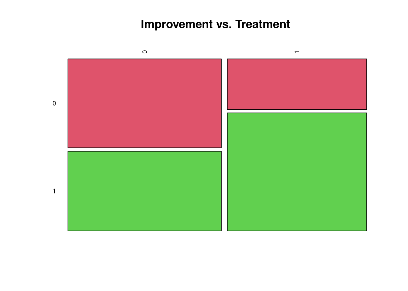
Compute chi-squred test
chisq.test (tbl)
    Pearson's Chi-squared test with Yates' continuity correction

data:  tbl
X-squared = 4.6626, df = 1, p-value = 0.03083
The Null Hypothesis is that treated and improved variables are independent.
In the above test the p-value is 0.03083, so at the significance level of 0.05 we can reject the null hypothesis